Poisson's Equation is the Most Powerful Tool not yet in your Toolbox

If you aren't used to staring at math, Poisson's equation looks a little intimidating:

What does \nabla^2f even mean? What is h? Why should I care?

In this post I'll walk you through what it means, how you can solve it, and what you might use it for.

Table of Contents

• What Does it Mean?
• When would I use this?
• How do I solve it?
• Dirichlet Boundary Conditions
• Optimize for speed
  • • Update in place
    • Overcorrection
• Visualizing the Outputs
• Poisson's Equation
  • • Why is Poisson's equation more useful?
• Neumann Boundary Conditions
• The Zoo of Boundary Conditions
• Superposition
• Conclusion
• Contact me

What Does it Mean?

Let's start by considering the special case where h=0. This is called Laplace's Equation:

It means:

Find me a function f where every value everywhere is the average of the values around it.

This problem statement applies in any number of dimensions, for continuous problems and for discrete problems. But in this post, when we talk about a function f we mean a 2D matrix where each element is some scalar value like temperature or pressure or electric potential. Like this:

If it seems weird to call a matrix a function, just remember that all matrices map input coordinates (i, j) to output values f(i, j). Matrices are functions that are just sparsely defined.

This particular matrix does satisfy Laplace's equation because each element is equal to the average of its neighbors. Here "average" means

Don't worry about how to define "average" on the edges for now and just focus on the center cell. Other examples that work, focusing on the center cell:

or

Examples that definitely do not satisfy the equation might look like

or

The central constraint--that each element is the average of its neighbors--means that any matrix that does satisfy Laplace's equation has a certain characteristic smoothness to it. A valid solution generally has no local minima or maxima.

When would I use this?

We use Laplace's equation to model any physical phenomenon where a scalar field is allowed to relax over time and we're only interested in the final state.

It makes sense that there can be no local minima or maxima--Any spot of metal on the plate that is hotter than all its neighbors will spread its heat to them and cool off. When all such small scale gradients have been exhausted and all the heat has flowed to equilibrium, we're left with a situation that satisfies Laplace's constraint.

So in practice, the problem we're trying to solve is that we have some huge matrix f that we know doesn't satisfy Laplace's equation. Maybe it describes:

• The initial temperatures measured on a radiator fin and we want to know the steady state temperatures
• The pressure distribution in a warehouse and we want to know how the wind will blow
• The distribution of electric potential across an acceleration gap in a particle accelerator and we want to know what the resulting particle trajectories will be

In all cases we're handed some initial, non-conforming state and we want to find the final state. Only the final state satisfies Laplace's equation.

How do I solve it?

Step through every cell and replace it with the average of the cells around it. Do this many times, until the values stabilize.

Again, for any interior cell we calculate the average as

Or, if you like a more formal notation:

So the interior cells are easy but what do we do at the edges and corners?

Laplace's equation on its own gives us no insight into how to handle the edge cases. We have to make an assumption based on our knowledge of the system. There are two common assumptions we can choose from:

Dirichlet Boundary Conditions: The values at the edges are fixed at some constant values that we impose.

Neumann Boundary Conditions: The derivative (or discrete difference) at the edges are fixed at some constant values that we choose.

Dirichlet Boundary Conditions

Dirichlet conditions are simpler to understand. Let's start with some function:

Where the bold values at the edges are fixed. Maybe the values represent temperature and the right edge is connected to some heat source while the other three edges are connected to heat sinks.

Let's loop over every cell and replace its value with the average of the cells around it. In Julia, something like:

function step(f::Matrix{Float64})
  # Create a new matrix for our return value
  height, width = size(f)
  new_f = zeros(height, width)
    
  # For every cell in the matrix
  for x = 1:width
    for y = 1:height
      if (x == 1 || x == width
        || y == 1 || y == height)
        # If we're on the edge,
        # just copy over the value
        new_f[y, x] = f[y, x]
      else
        # For interior cells,
        # replace with the average
        new_f[y, x] = (
          f[y-1, x] + f[y+1, x] +
          f[y, x-1] + f[y, x+1]) / 4.0
      end     
    end
  end
  return new_f
end

f = zeros(6, 6)
f[1:6, 6] .= 1.0  # Set the right side to ones
display(f)

for step_number = 1:3
  println("\n")
  global f = step(f)
  display(f)
end

The output looks like:

And if we run it long enough it'll stabilize to something like:

Go ahead and check it! For every interior cell, the value is equal to the average of the values around it! (At least approximately)

In its simplest form, solving Laplace's equation is as easy as just calculating a bunch of averages over and over again. You could program this yourself in whatever language you choose.

The only problem with this approach is that it takes a long time.

Optimize for speed

This section is interesting but optional! Skip to Visualizing the Outputs if you don't care about speeding up our solver by 70x!

We generally run a relaxation until the values stabilize. We set some threshold like 1e^{-10} and if all updates are smaller than the threshold, we say it has stabilized.

We can add this threshold check and run the loop until stablization. For this tiny example it takes 97 steps to converge.

If we want to run a higher-resolution simulation on say a 100 \times 100 square grid, that takes 28,851 steps.

Update in place

The first optimization is to just update the values in place rather than creating a new matrix for each step. See example3.jl for a reference implementation. This trick allows information to flow faster because cells that have already been updated can contribute their new value to cells that have yet to be updated.

For example, if we start with

We arrive at

In just a single step! Though we are still far from convergence, heat from the left edge is able to travel across the entire matrix in a single step. In our original implementation, heat could travel a maximum of 1 cell per step.

Just by making this one change the number of steps required for convergence drops from 28,851 to 15,139 with no loss of accuracy!

If you want to read more about this optimization, it is called the Gauss-Seidel method.

Overcorrection

The difference between a cell's current value and the value we're about to replace it with is called the correction. If we purposefully overcorrect, we can reach convergence faster.

In Julia, something like

old_value = f[y, x]
average = (f[y-1, x] + f[y+1, x] + f[y, x-1] + f[y, x+1]) / 4.0
correction = average - old_value
f[y, x] += correction * overcorrection_factor

The overcorrection trick profoundly boosts performance:

With an overcorrection factor of 1.94, it only takes 407 steps to converge! Down from 15,139!

The optimal overcorrection factor will vary with the size of the matrix, the boundary conditions, and the initial internal cell values. 1.94 is a great starting value but you'll need to tune it yourself if you want optimal solving speed on a particular problem.

This optimization is called Successive Over-Relaxation.

Visualizing the Outputs

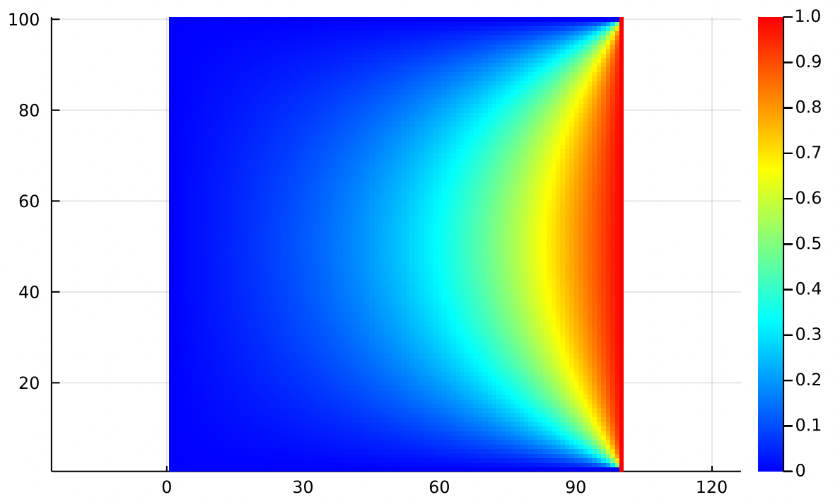
Instead of looking at f as a table of numerical values between 0 and 1, let's interpret the matrix values as pixel brightness:

This is the solution to our original boundary conditions of 0 everywhere and 1 on the rightmost boundary, just scaled up to 100 \times 100 cells. If the value in question is heat, this output matches our expectation that heat flows in from the edge and heats up just the right side of the grid.

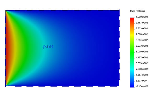
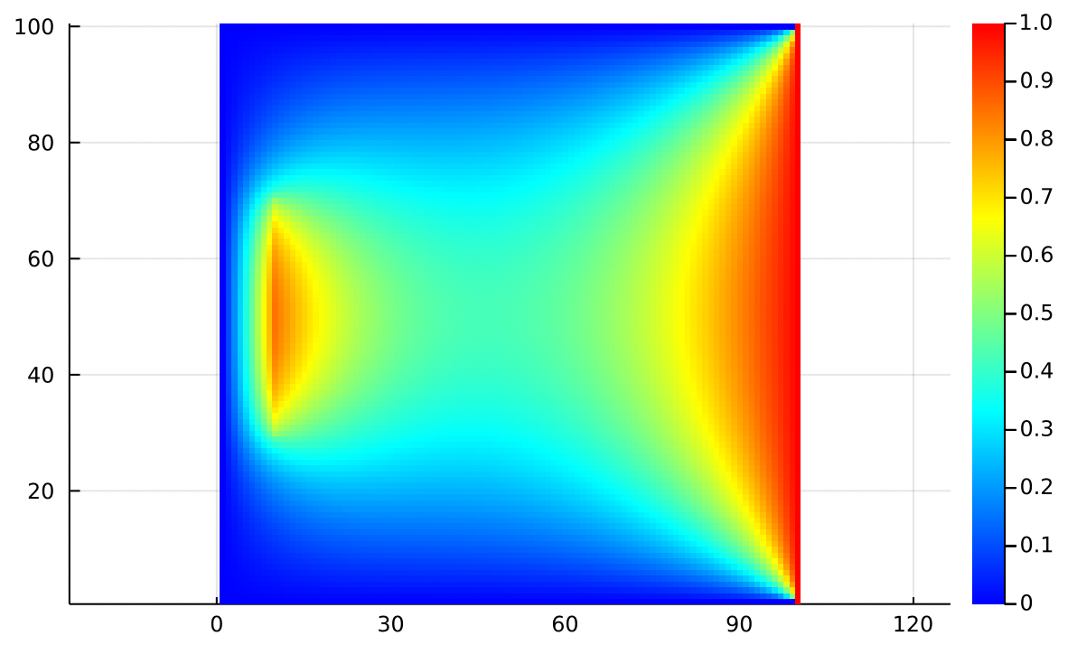
It is customary when simulating heat flow to use a wacky color palette where red is hot and blue is cold, with all kinds of intermediate colors in between:

I think this colormap is a little tacky, but it's what you find in all the textbooks. Maybe it helps you see the fine structure of the answer better. Maybe it just subjectively feels more like heat because we're used to seeing red as hot. Use whatever colormap helps you the most.

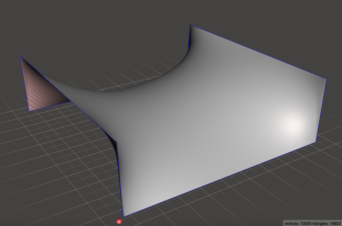
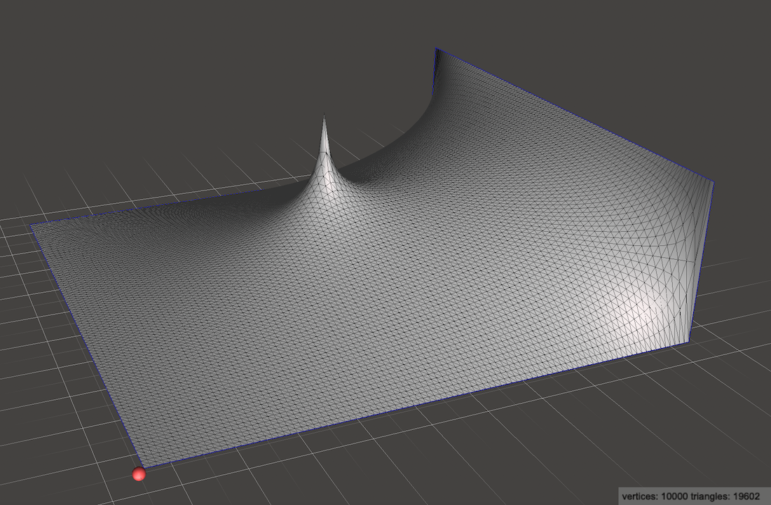
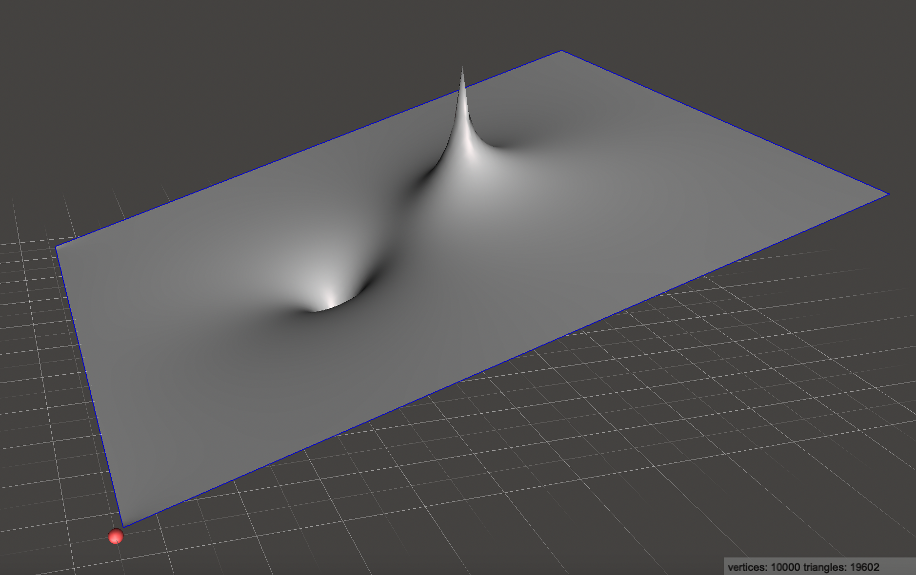
Instead of living in 2D and making images, we can interpret the values as heights and build a 3D surface:

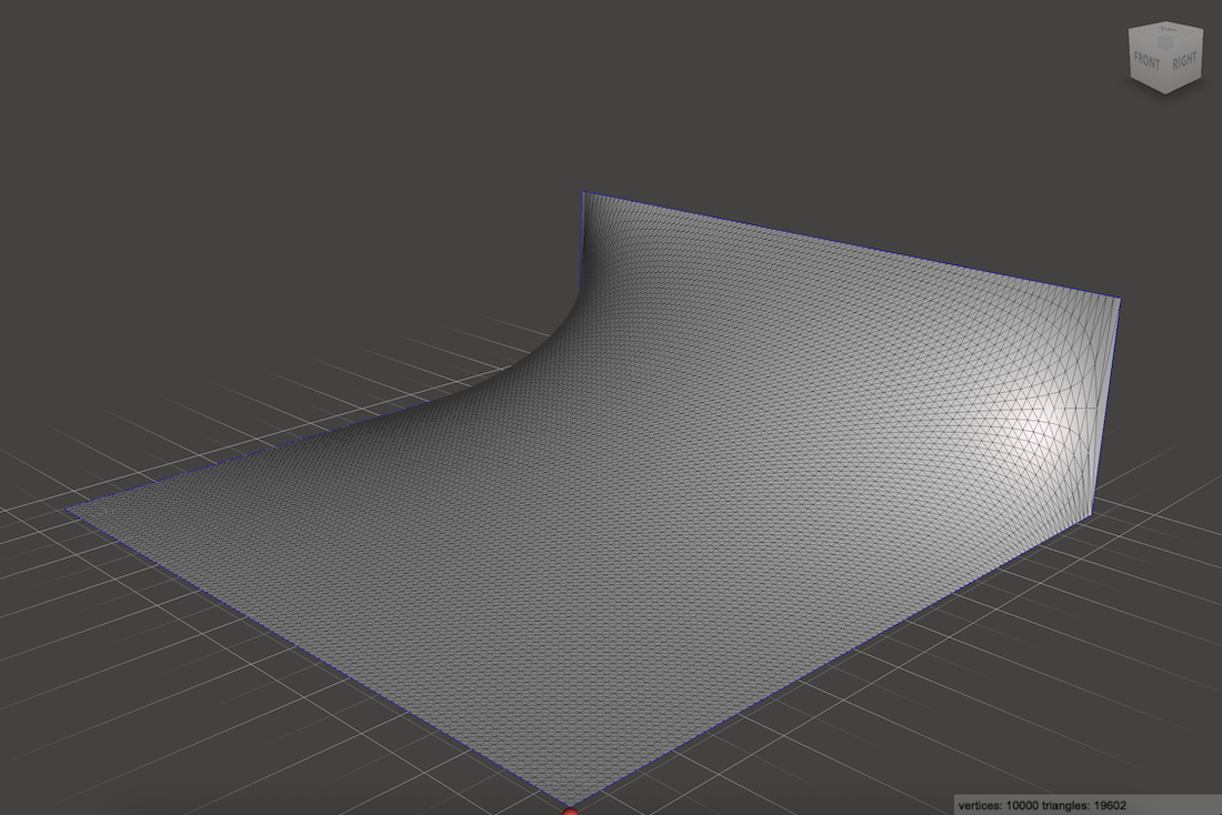
(Here I've exaggerated the height by 30x just to see it better)

This is a common way to visualize electric potential functions because it is super easy to interpret: a negatively charged particle, if left to drift through this potential field, would roll downhill like a marble on a ramp. A positively charged particle, which is just a negatively charged particle with its time dimension reversed, would roll uphill. This gives us everything we need to know to plot the trajectory of a charged particle through an acceleration gap!

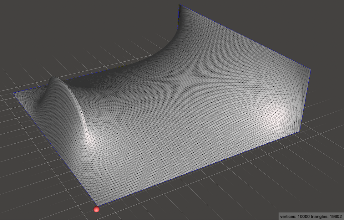
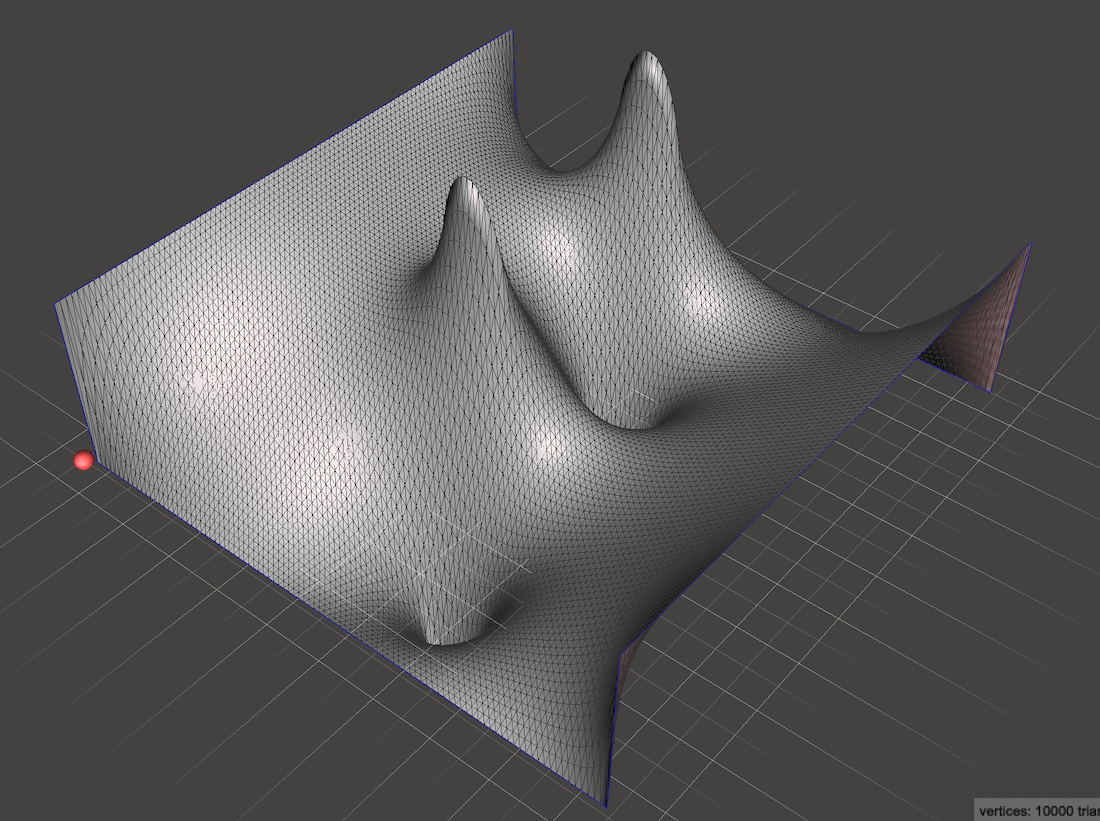
A slightly more interesting example would be to charge both the side walls to create a saddle:

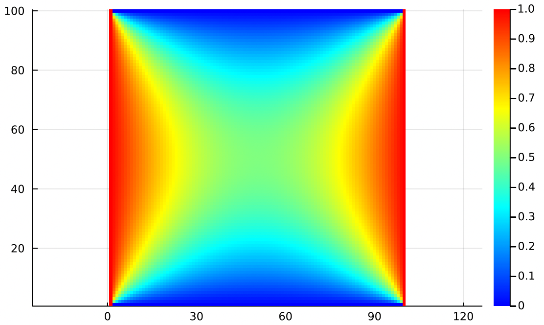
Looking at the ramp it is obvious that a marble should roll down from the left or right edges and then fall off the top or bottom edges. To visualize the paths better we might draw little arrows which everywhere point in the direction most downhill.

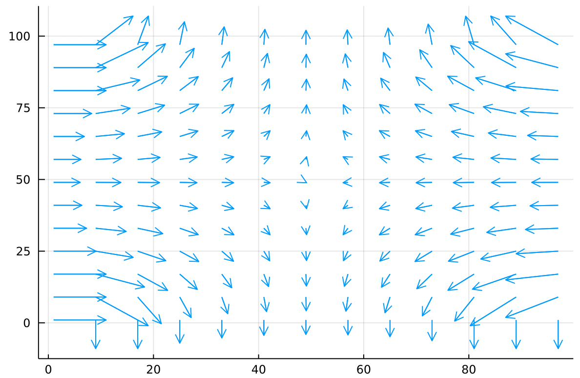
This field full of arrows all pointing downhill is written

And is pronounced "negative grad f" or "the negative gradient of f". The gradient is very easy to calculate, we just find the difference between each cell and the cell to its right. This gives us the x component of the gradient. Then we calculate the difference between each cell and the cell below it. This gives us the y component of the gradient. The full gradient, defined at each cell, is just the vector you get by adding the x and y components together.

The gradient produces arrows which point uphill, from cold to hot. The negative gradient is just the gradient with a minus sign in front of each x and y component, so it points downhill.

Using -\nabla f we can simulate stepping a particle through this field to produce its trajectory, a problem similar to numerically integrating an ordinary differential equation.

Poisson's Equation

At this point we've got a pretty good handle on Laplace's Equation:

And we're ready to level up to Poisson's Equation, which is almost identical but much more useful:

It means:

Find me a function f where every value everywhere is the average of the values around it, plus some pointwise offsets.

In the land of matrices, this means we now have to deal with a matrix h which is the same shape as f, and is full of user-specified offsets.

The modification to our code is straightforward. Instead of replacing f(i, j) with the average of the cells around it, we replace f(i, j) with the average of the cells around it plus an offset h(i, j), which is just the (i, j) value of the matrix h. That's really it!

To solve Laplace:

average = (f[y-1, x] + f[y+1, x] + f[y, x-1] + f[y, x+1]) / 4.0
f[y, x] = average

To solve Poisson:

average = (f[y-1, x] + f[y+1, x] + f[y, x-1] + f[y, x+1]) / 4.0
f[y, x] = average + h[y, x] / 4.0

Where the extra factor of \frac{1}{4} comes from the fact that in 2D, a square cell has four neighbors. In 3D that factor is \frac{1}{6} because a cube has 6 neighbors. Can you intuit what that factor is for a 4D hypercube?

To accommodate overrelaxation we write it:

delta = (f[y-1, x] + f[y+1, x]
          + f[y, x-1] + f[y, x+1]
          - 4 * f[y, x]
          + h[y, x]) / 4.0
f[y, x] += 1.94 * delta

And again we achieve excellent performance. When h=0, our simulation simplifies to just solving Laplace's equation.

Why is Poisson's equation more useful?

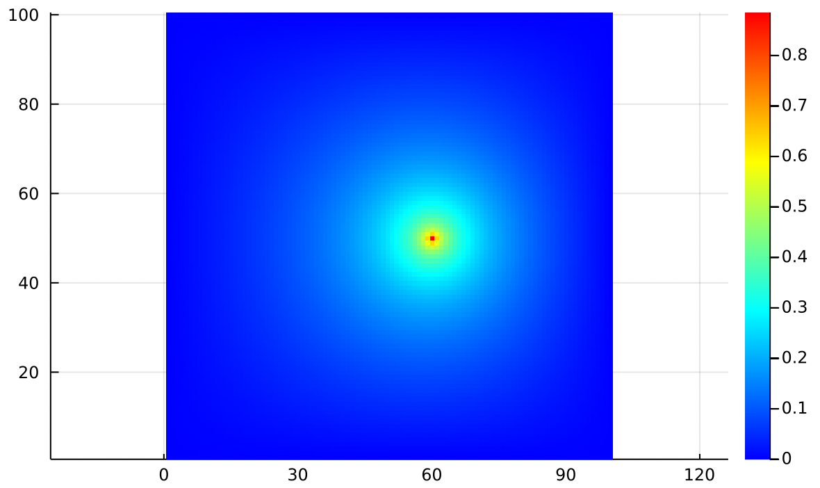
If we use an h which is everywhere zero, but at the center has a single -1, we are modeling adding a single heat source at the center of the metal plate:

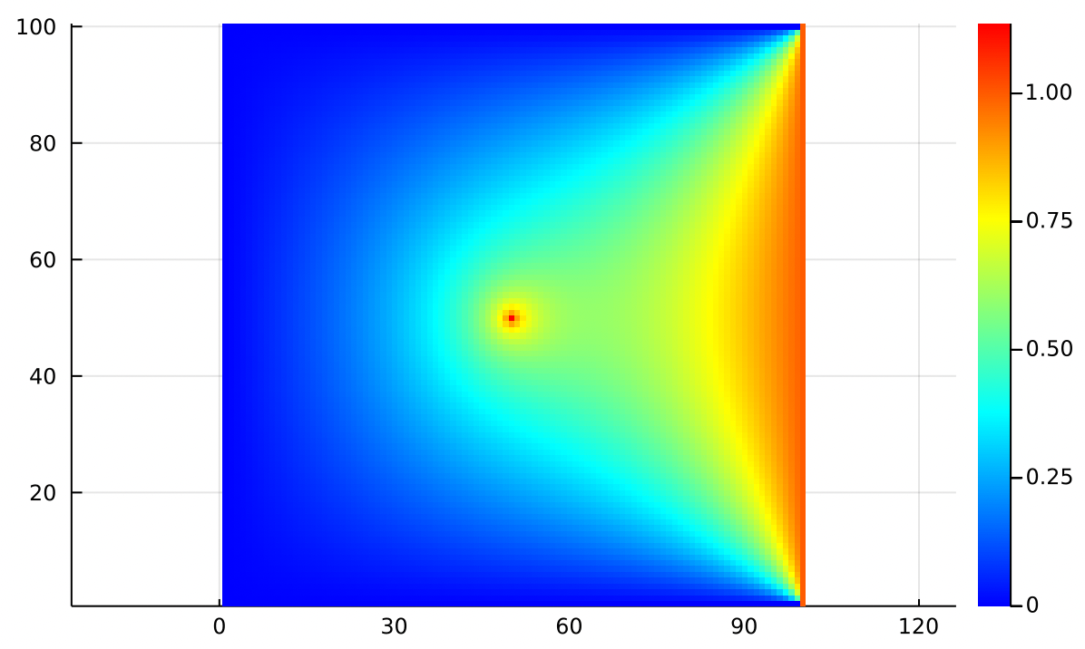
Just by modifying h we can encode any distribution of heat sources and sinks anywhere in 2D space, rather than being limited to only having sources and sinks at the edges of the plate.

This extra matrix h gives us tremendously more modeling freedom! We can add a line source instead of a point source:

Or any arrangement of heat sources and sinks that we desire!

Note that in specifying Dirichlet boundary values, we were specifying the temperature directly. "The right edge is 1 degree and the left edge is 0 degrees".

In specifying h values, we're saying something relative about how that point compares to its neighbors. "The center point is hotter than the average of its neighbors by 1 degree". So what we're actually controlling there is not the temperature directly, but the sharpness of the spike that it creates.

Maintaining a constant temperature difference between points means that heat must be flowing constantly from the hot point to the colder points. That's why we think of a h as describing the locations and powers of heat sources and sinks.

Neumann Boundary Conditions

Very often, imposing Dirichlet boundary conditions is unphysical. In real life how could you ever guarantee fixed temperatures on the entire boundary of a metal plate?

In many real world examples we know the distribution of heat sources and sinks (h), and we know that at the edges no heat can flow. Imagine our metal plate surrounded on all sides by a perfect thermal insulator. No heat can flow into a perfect insulator, and it would be unphysical for heat to accumulate at the boundary, so the difference in temperatures for points near the boundary must be zero.

Being surrounded by perfect insulators is not a statement about the temperature at the edges, it is a statement about the spatial derivative of temperature at the edges. Namely, that the derivative must be zero across the boundary.

Neumann Boundary Conditions enforce that heat is not allowed to flow through the boundaries.

The clearest way to simulate this condition is to just mirror the function across all boundaries and treat edge cells the same way you treat interior points. So the new situation looks like this:

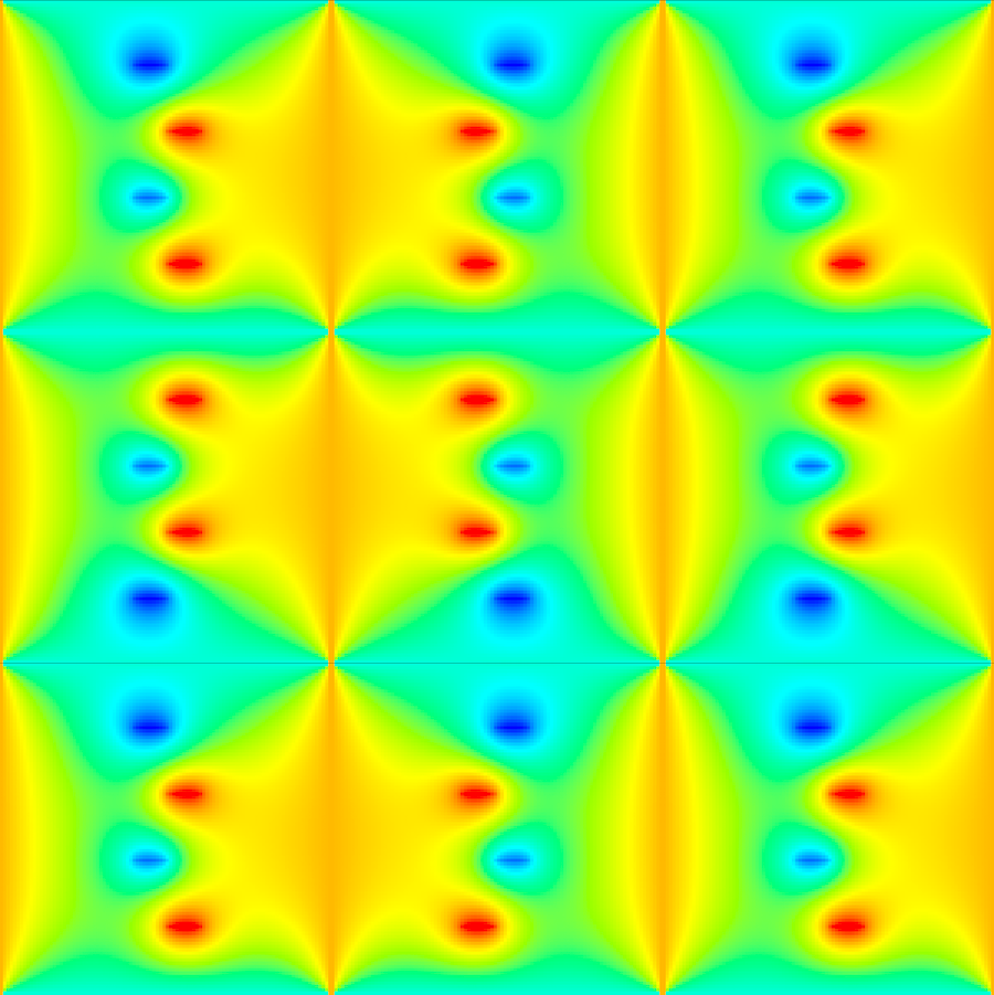
Where we're only interested in the centermost copy, and we need to smooth over all the edges so that the mirrored copies blend seemlessly into each other. Of course we don't need to actually copy the matrix 9 times, we can just simulate mirroring across boundaries like this:

# These are the indices that we pull from for the inner cells
y_up = y - 1
y_down = y + 1
x_left = x - 1
x_right = x + 1

# But if we're on a boundary, we have to simulate reflection
if x == 1; x_left = x + 1 end
if x == width; x_right = x - 1 end
if y == 1; y_up = y + 1 end
if y == height; y_down = y - 1 end

delta = (f[y_up, x] + f[y_down, x]
          + f[y, x_left] + f[y, x_right] - 4 * f[y, x] + h[y, x])
f[y, x] += 1.94 * delta / 4.0

See poisson2.jl for the full source code.

Looking back, we notice that Dirichlet boundaries often produce sharp ramps at the edges of the simulation. In contrast, Neumann boundaries always produce smooth, flat edges:

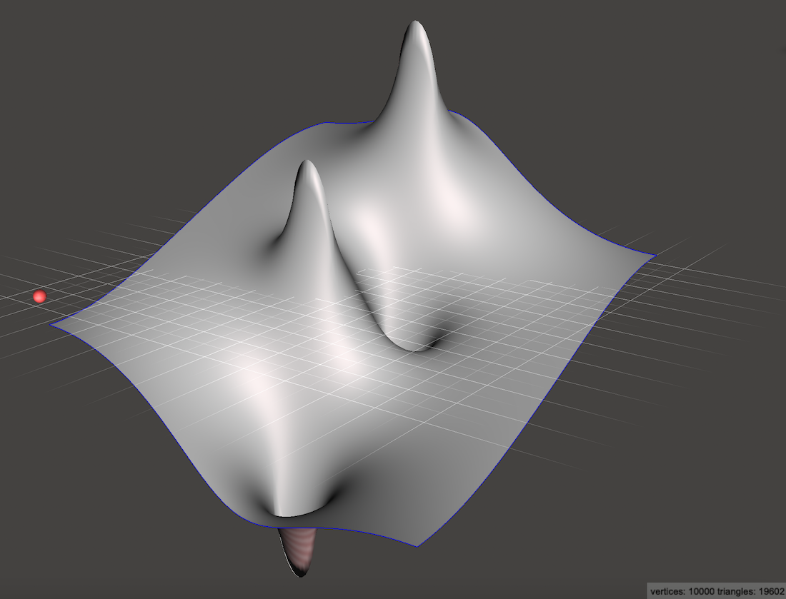
If you place a marble at rest on any edge of that heightmap, it will not tend to roll off the edge. It may roll downhill along the edge, but it won't fall. That's because on the left and right edges, the gradient from left to right must be zero. Along the top and bottom edges, the gradient from top to bottom must be zero.

In the case of fluid flow in a closed container, Neumann conditions mean that fluid cannot flow through the walls of the container.

One last condition to keep in mind is that if you only have Neumann conditions, Poisson's equation is only uniquely solvable if you insist that \int h=0. In our case that means that the sum of every element of h must come out to be exactly zero: \sum h=0. This restriction does not apply to Dirichlet conditions.

The Zoo of Boundary Conditions

Earlier I said that Poisson's Equation does not on its own tell us what to do at the boundaries and that we have to impose some kind of boundary conditions based on our physical understanding of the problem. In many cases the physics of your situation will make it clear which boundary conditions are appropriate, but there are a lot more than two options.

You should know that Dirichlet conditions can be specified as any real values, not just the 0 and 1 seen in the examples here. They can also vary along the length of the edge to give linear gradients, sharp discontinuities, really anything you can imagine. This can be helpful in electrostatics where certain parts of the boundary are held at known voltages.

Similarly, Neumann conditions can be specified as any real numbers, not just the 0 shown above. This is useful in magnetostatics problems where you know the desired magnetic field strength and you need to solve for the magnetic flux density along the interior profile of the magnet.

Also, sometimes it is appropriate to specify both the value and the spatial derivative along a particular boundary. This is called a Cauchy boundary. This doesn't come up much with Poisson's Equation, but it is possible.

Occasionally you might need to use Neumann conditions on some parts of the boundary and Dirichlet conditions on other parts, though the code for this gets a little more intricate. This is called a Mixed boundary.

Lastly you might end up in a situation where you don't know the fixed value at the boundary and you don't know the derivative at the boundary, but you do know something about a weighted combination of the two. This is known as a Robin boundary and it is used in electromagnetics when what you know is something about the impedance of the boundary, or when you're modeling multiple types of heat flow which together sum to some value.

Boundary Condition are a deep subject. Half the battle is just knowing what exists.

Superposition

This may seem surprising and I won't try to prove it here, but you can add together solutions to get new solutions!

If f and g are two functions both individually satisfying Poisson's Equation, then their sum f + g is also a solution.

For example, using Dirichlet boundaries we can fix the left side at 0 and the right side at 1, with a linear ramp on top and bottom. The solution f is just a linear ramp:

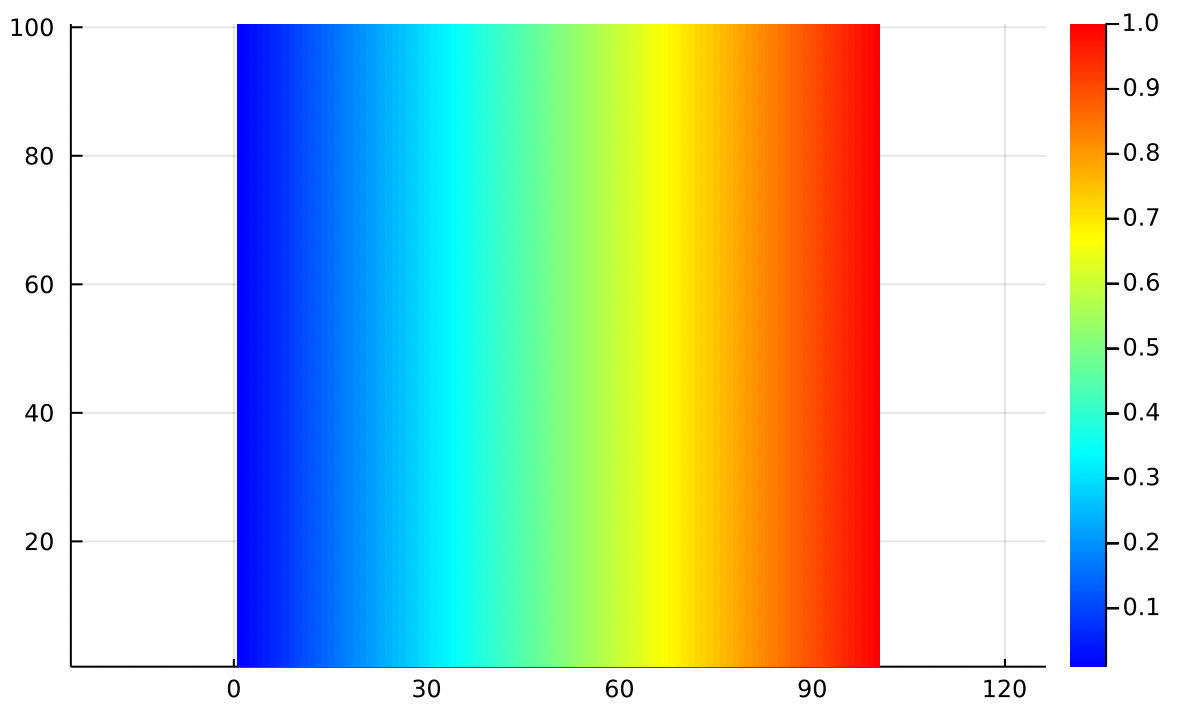
In aerodynamics we might think of f as the aerodynamic potential. The gradient of the aerodynamic potential gives us the velocity field:

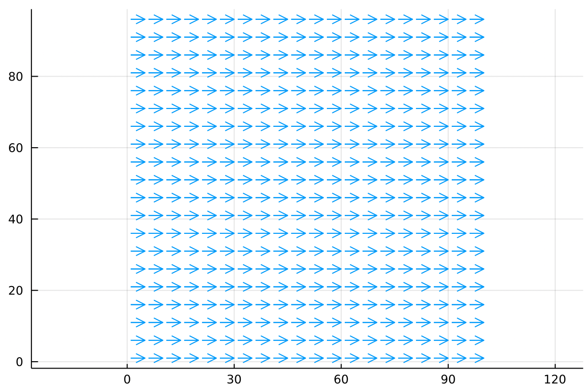
Where we can interpret the arrows as the wind. This particular potential function models a uniform airflow from left to right. Remember that the positive gradient points uphill from blue to red.

Separately we can create a point source of air, with Dirichlet boundaries fixed at zero. Think of this like a hose injecting air into a sealed, square chamber.

The air nearest the point source moves fast but slows down as it gains some distance. The velocity drops to zero at the edges because this chamber is sealed.

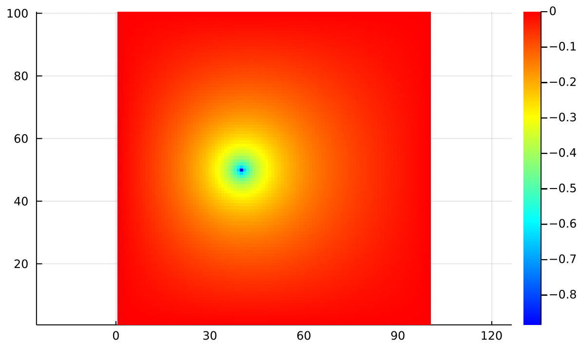
In the same vein, we can make a point sink of air with the same sealed boundary conditions. This is a vacuum hose sucking air out of a sealed chamber:

Again the main feature is that the arrows get longer as they get closer to the point sink.

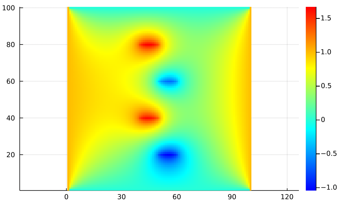
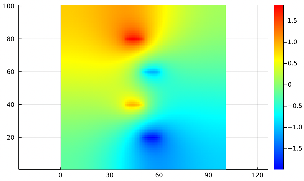
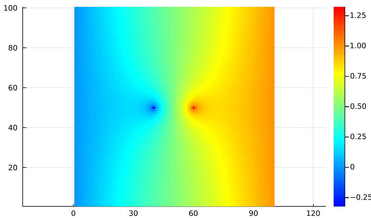
All three of these are valid solutions to Poisson's equation, so we can just add them together to end up with a new solution which has elements from each! The combined potential function looks like:

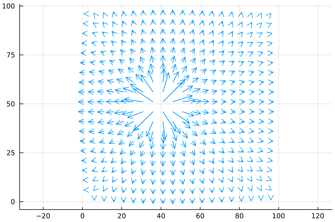
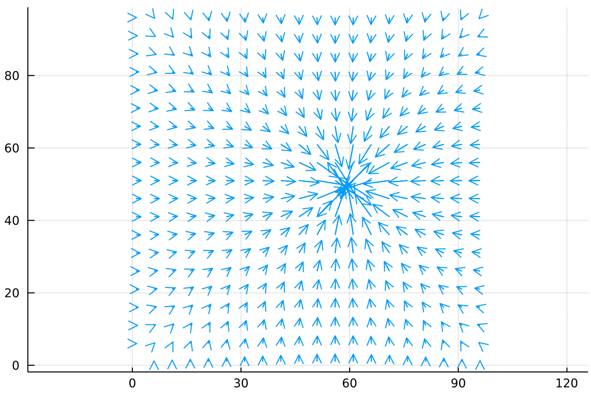
Remembering that for the gradient, arrows point uphill:

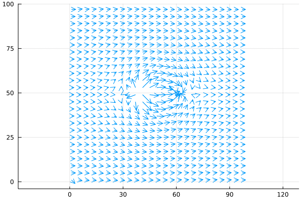
The flow field we've created is very interesting! From a distance, uniform flow dominates the velocity field, but there are two localized regions which look like a source and sink. If we trace the velocity field carefully, we actually find that every single bit of air blown out of the source gets absorbed by the sink! This is no coincidence as they were created to be equal and opposite strengths.

It might not be obvious at first glance but we can draw an oval on this flow field which is tangent to the velocity field at all points. This corresponds to a watershed boundary in the heightmap.

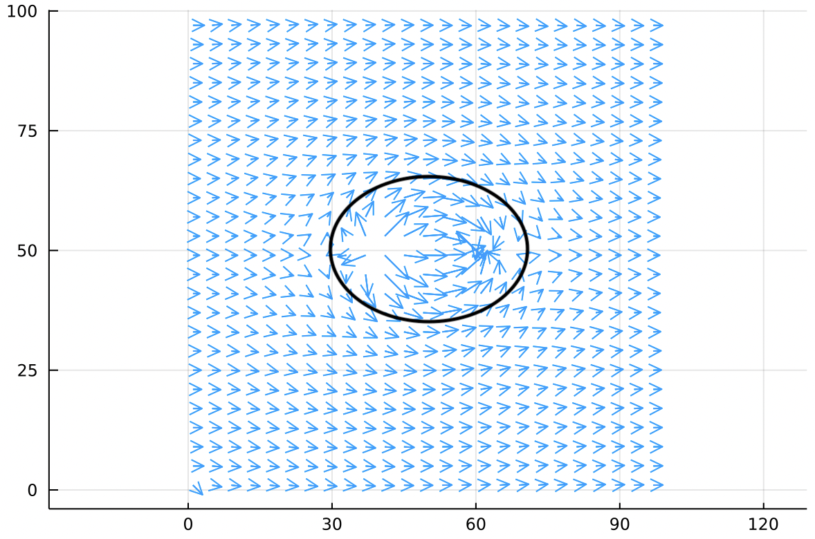
This oval (called a separatrix) has the special property that no wind flows through it at all. It acts just like a solid surface. We have already assembled a reasonably accurate simulation of how air flows around an ellipse in some confined space like a wind tunnel!

From here we could use Bernoulli's equation to find the pressure distribution, which we could integrate over the surface to find drag and lift and so on. With a few tweaks we could simulate rotational flow, vortex panels, real wing profiles, and so on.

With just a few simple building blocks we're already edging up on real computational fluid dynamics. All this just by adding up some matrices!

One word of caution: When you add solutions in this way, realize that you're adding the boundary conditions as well. If you're just dealing with Dirichlet boundaries all around, this makes sense. But if you're trying to add solutions together that have incompatible boundary conditions, things start to get very tricky very fast and it possible to end up with something that is nonphysical. You need to thoroughly understand your domain to know if you're making a misstep.

Conclusion

Poisson's equation comes up in many domains. Once you know how to recognize it and solve it, you will be capable of simulating a very wide range of physical phenomena.

The knowledge from this post is a jumping off point into many, much deeper fields.

For applications we've already discussed steady-state temperature distributions, electrostatics and magnetostatics, and computational fluid dynamics. But these same tools are also used in geophysics, image processing, caustics engineering, stress and strain modeling, Markov decision processes, the list goes on!

I want to mention that this entire post has treated f like it has to be a matrix of finite size, because that's very common in engineering. But f can be any continuous function that extends out to infinity. The tools available in that case are a little different but much of the knowledge, especially the technique of solving simple problems and adding them together to solve complex problems, is the same.

Speaking of superposition, you should know that Laplace's Equation has a close cousin called the Biharmonic Equation:

Which is widely used in modeling quantum mechanics. The name comes from the fact that solutions to Laplace's equation are called Harmonic Functions.

Lastly I need to stress that I only illustrated three highly-related ways of solving Poisson's equation. There are many ways to solve it, including multi-grid approaches that solve the problem in stages or in parallel, approaches based on fast fourier transforms, and a family of solvers called Galerkin methods. There are dozens more, all with their own strengths and weaknesses. Successive overrelaxation is just the easiest to understand.

Likewise there are countless extensions to the problem to deal with non-uniform grid spacing, non-cartesian coordinate systems, higher dimensions, and a hundred other variations. Each of these extensions has its own library of algorithms that can be used to solve it.

I hope that recognizing Poisson's equation and how to solve it will help you feel equipped to tackle a broad range of problems that you might otherwise not have tackled.

Contact me

If you wanna talk about Poisson's Equation and its million uses, hit me up on twitter @mferraro89 or email me at mattferraro.dev@gmail.com.