Hiding Images in Plain Sight: The Physics Of Magic Windows

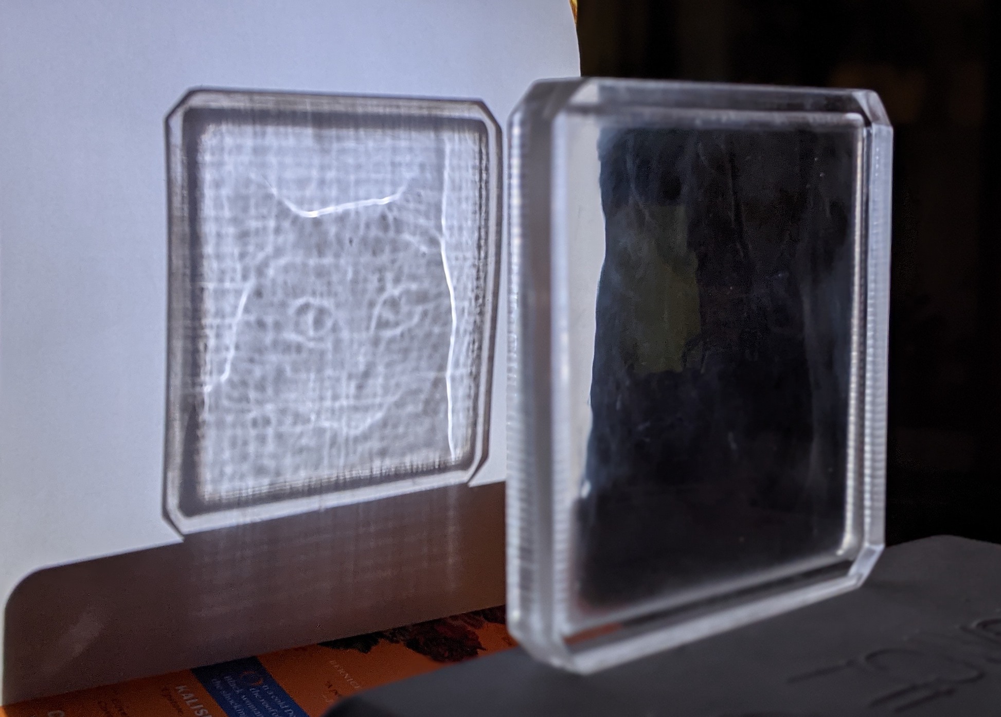
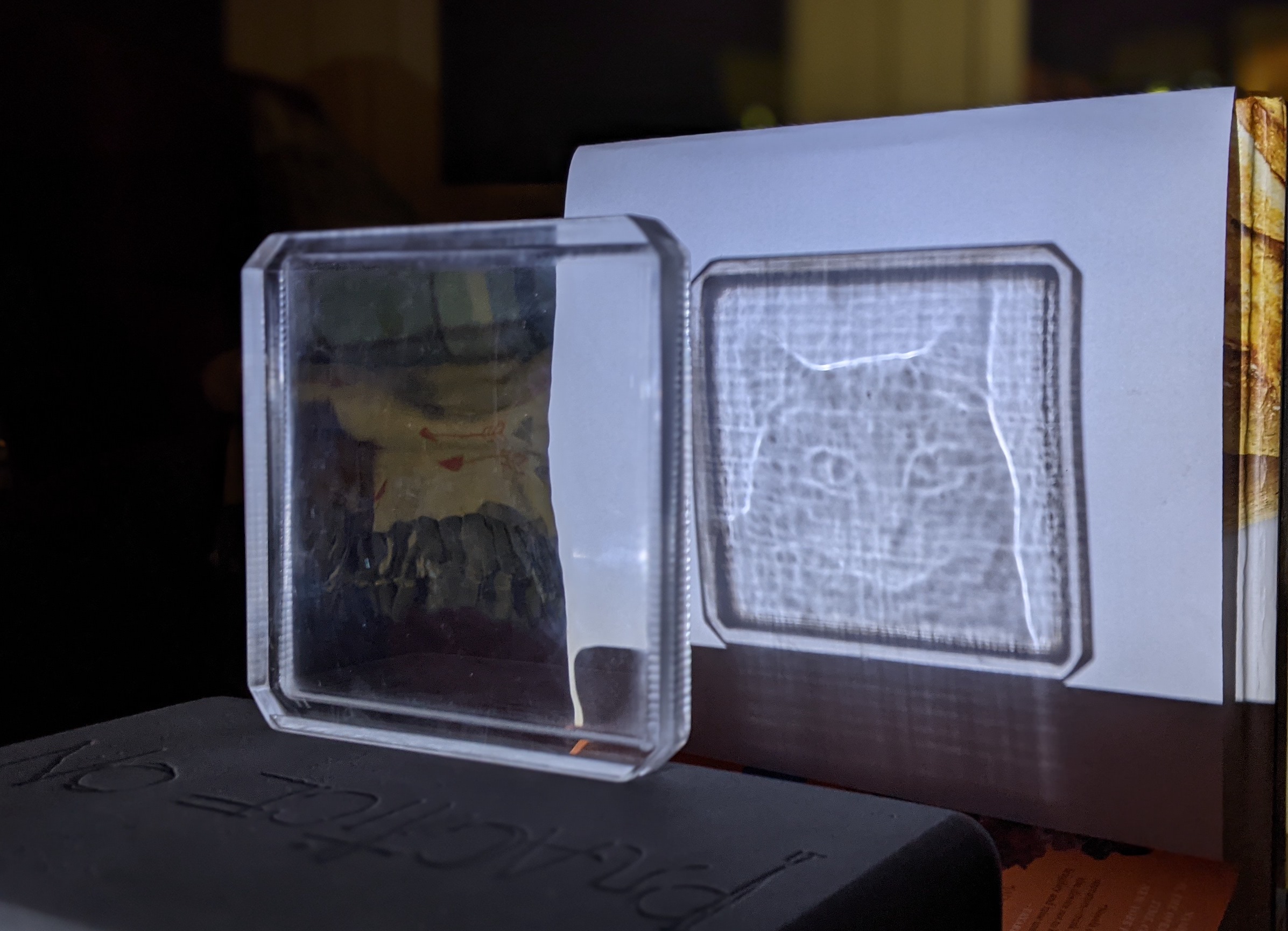
I recently made a physical object that defies all intuition. It's a square of acrylic, smooth on both sides, totally transparent. A tiny window.

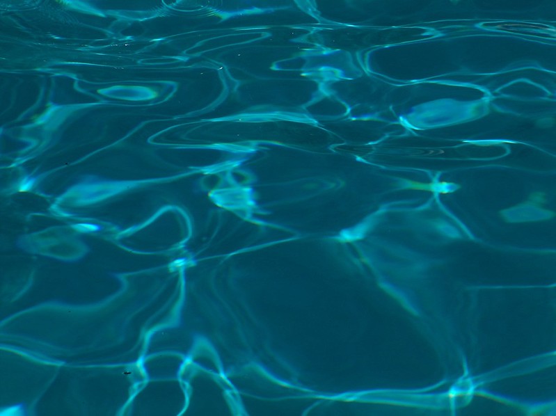
But it has the magic property that if you shine a flashlight on it, it forms an image:

And if you take it out in the sun, it produces this 3D hologram:

This post describes the math that went into making the object, and how you can create your own.

But first: How is this even possible?

Let's focus on the 2D image before talking about the hologram.

The physical phenomenon we're looking at is called a caustic.

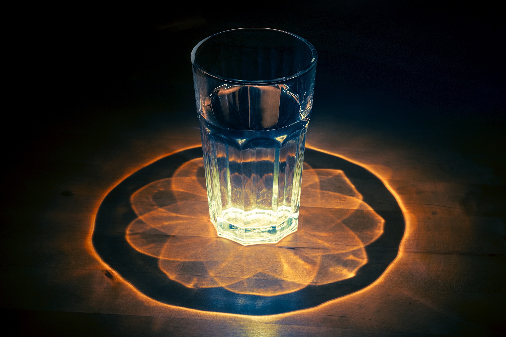
Caustics are the bright patches of light we see when illuminating a transparent object. All the photons that don't pass directly through the object are what form the object's shadow. All those photons still have to go somewhere; they contribute to the caustic pattern.

The most interesting aspect of caustics is that they arise from even the tiniest of variations in surface flatness. Even the gentlest waves on the surface of a pool form powerful lenses that cast intense caustics on the floor below.

The reason my acrylic square can form an image is because I've distributed just the right amount of concavity and convexity into the surface so that the refracted light forms a caustic image.

To gain some intuition for how it is done, consider a traditional convex lens:

This lens forms the simplest possible caustic. If all the incoming light is from a single, very distant light source like the Sun, this lens focuses all of its incoming light into a single point. The caustic image from this lens is dark everywhere with one very bright spot in the center.

Zooming in on one small section of the lens we notice a few properties:

1. The overall thickness of the lens does not have a direct impact on the outgoing ray angle. We could add material to the left side of this lens and nothing would change. The first transition, from air to glass, can be entirely ignored.
2. The angle between the incoming light rays and the glass-air boundary has a strong effect on the refracted ray angle.
3. Whether two rays converge or diverge is controlled by how curved the lens is where the glass meets the air

In other words, the height of the glass h(x) is not on its own important. But the slope of the glass, \frac{\mathrm{d}h}{\mathrm{d}x}, gives us the outgoing ray angle via Snell's law. Where rays converge the image is brighter than the light source. Where rays diverge the image is darker. Therefore the brightness of the image (at that point, where the rays fall) is related to \frac{\mathrm{d}^2h}{\mathrm{d}x^2}.

The thickness of my acrylic slab varies across the entire xy plane, so I'll call it h(x,y) and we'll think of it as a heightmap.

By controlling \nabla h = (\frac{\partial h}{\partial x}, \frac{\partial h}{\partial y}), and \nabla ^2 h = (\frac{\partial ^2 h}{\partial x^2} + \frac{\partial ^2 h}{\partial y^2}), we can steer all of our incoming light to the correct locations in the image, while contributing the right brightness to make it recognizable. By making some simplifying assumptions we can guarantee that the resulting heightmap will be smooth and continuous.

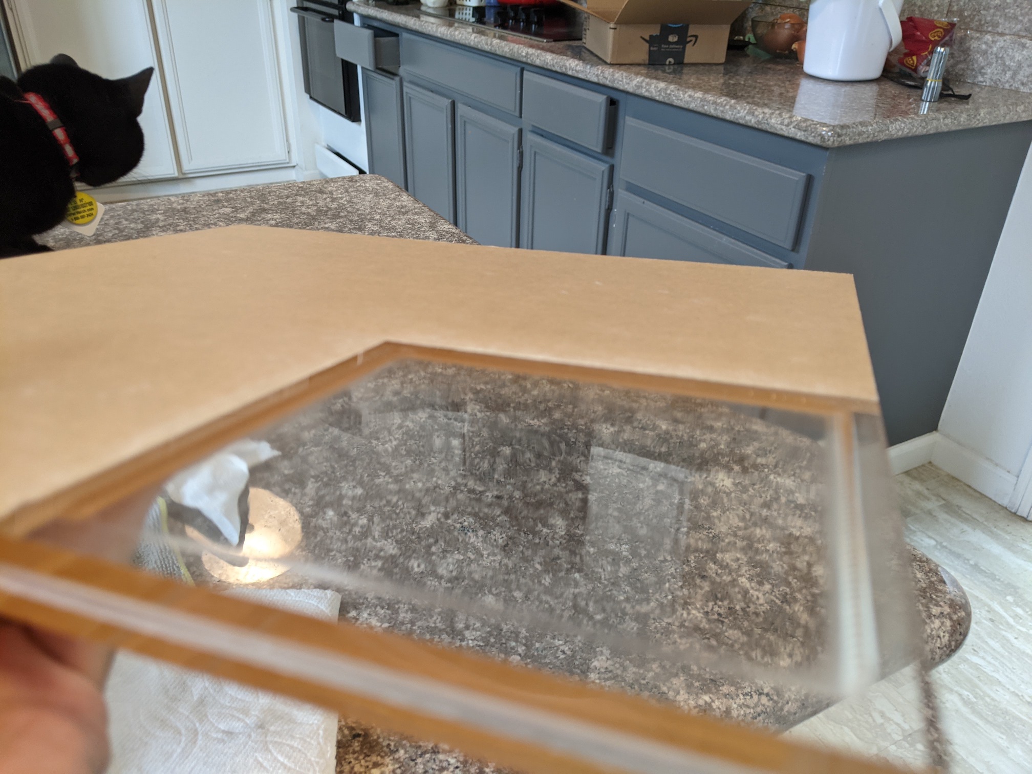
For the Magic Window shown above, the total height variation over the 10cm \times 10cm surface is about 2.0mm.

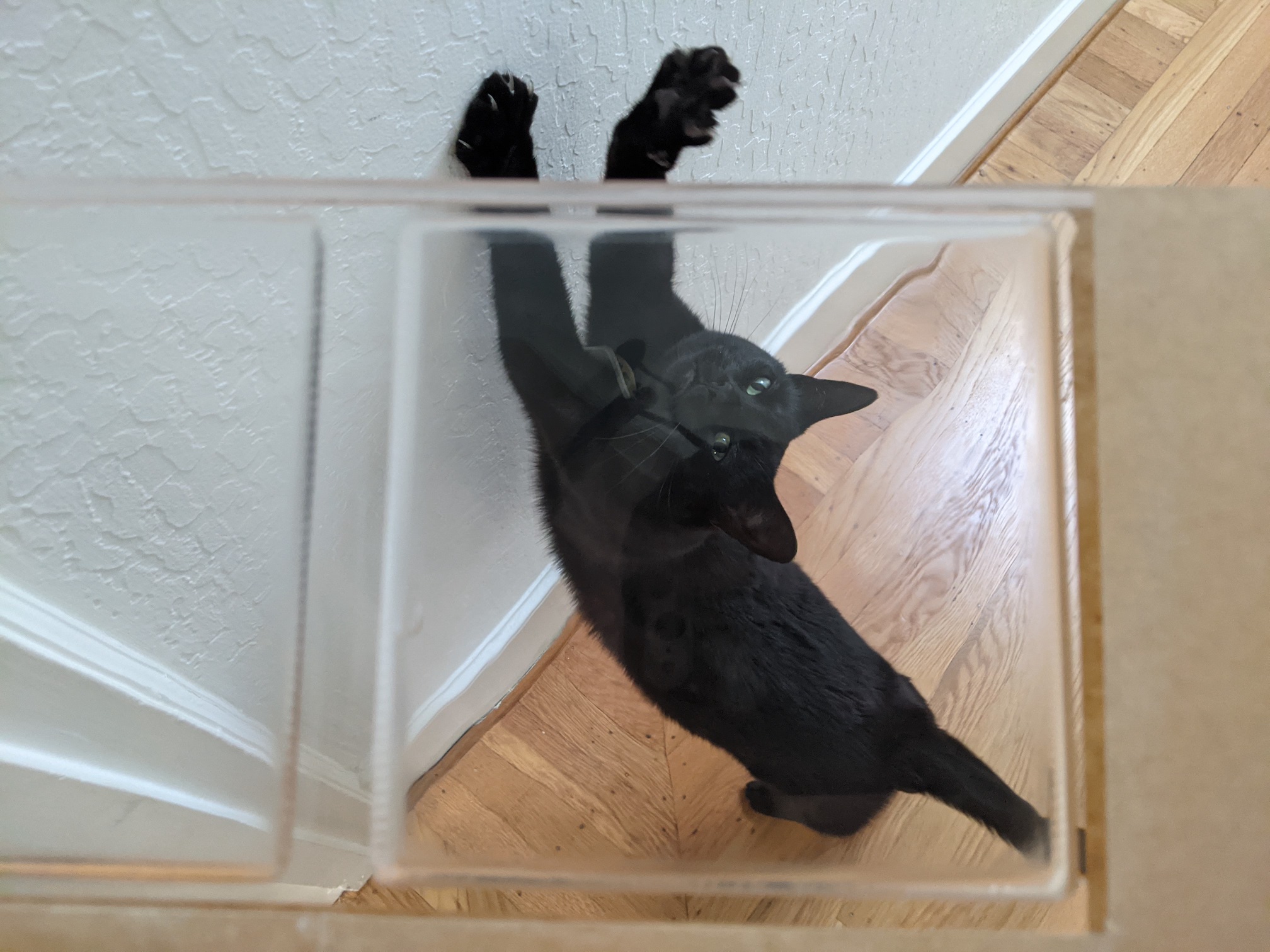
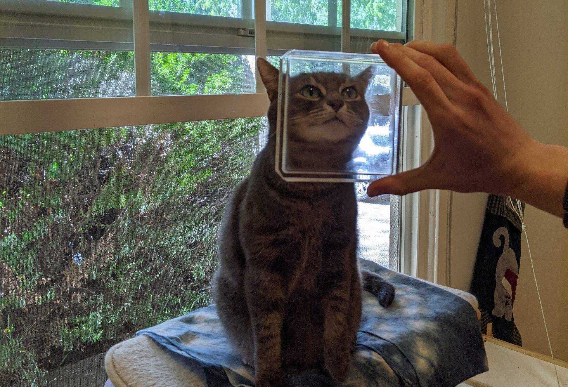
See how the slight variations in surface height distort the straight line of the floor moulding? Our Magic Window works like any other lens—by bending light.

Table of Contents

• Formulating the Problem
• Steps to a Solution
• Morphing the Cells
  • Computing the Loss
  • Stepping to Reduce Loss
• Snell's Law and Normal Vectors
• Finding the Heightmap
• Manufacturing
• Acknowledgements
• My Code
• Licensing
• Contact me
• One Last Thing

Formulating the Problem

We want to find a heightmap h(x,y) whose caustic image has brightness b(u,v), equal to some input image. To achieve this we can imagine a grid of cells, akin to pixels, on the surface of the acrylic lens. Here each "pixel" on the lens corresponds to a pixel in the image. Image pixels and their corresponding lens-space "pixels" are labeled with shared (i, j) coordinates.

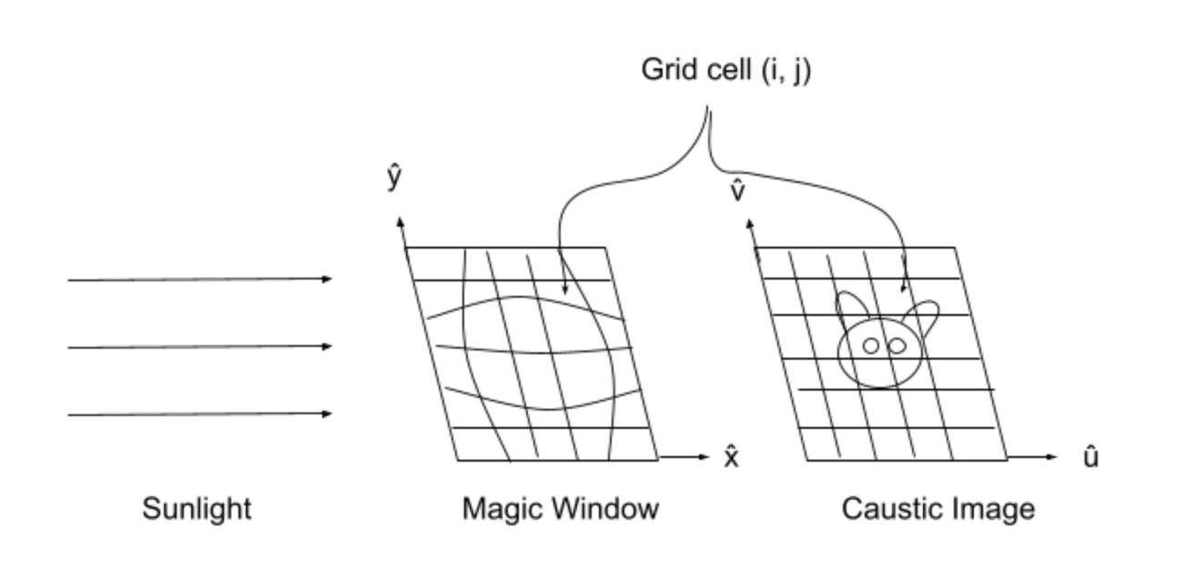
Remember that (i, j) are integers labeling the column and row of the pixel, whereas (x, y) and (u, v) are real numbers measured in something like meters or inches.

Steps to a Solution

Step 1: We morph the cells on the lens, making them bigger or smaller, so that the area of lens cell (i, j) is proportional to the brightness of image cell (i, j). The resulting lens grid is no longer square—lots of warping and skew have to be introduced to maintain continuity. This step is by far the hardest part and must be solved iteratively.

Step 2: For each cell (i, j) we need to find the angle from the lens cell to image cell and use Snell's law to find the required surface normal. This step is straightforward geometry.

Step 3: Integrate all the surface normals to find a continuous heightmap h(x,y). We're back to iterative methods here, but if we apply certain contraints to how we solve step 1, this step is actually fast and easy.

Morphing the Cells

For an image with n \times n pixels, the lens grid will need (n+1) \times (n+1) points, so that each cell in the lens grid is defined by four points. Technically we should adopt yet another coordinate system to label the points in the lens grid since they are distinct from the cells in the lens grid, but I think it's easier to just reuse (i, j) and we can say that for grid cell (i, j), the point in the upper left is defined as grid point (i, j).

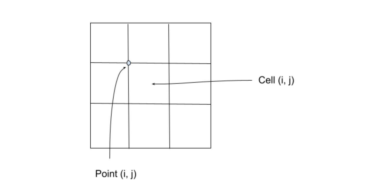
This leaves us with one row and one column of extra grid points along the bottom and right edges, but that will be trivial to deal with when it comes up.

Each point in the lens grid (i,j) has an (x, y) coordinate. A point's (i, j) coordinates never change but the (x, y) coordinates will change as we morph the cells more and more.

Computing the Loss

Given the (x, y) locations of all the lens grid points, simple geometry lets us calculate the area of each lens grid cell. Of course at first every cell has the same area, but that will change as soon as we start morphing things.

The condition we want is that every lens grid cell (i, j) has an area which scales with the brightness of image pixel b(i, j).

Area and brightness are not compatible units so it is helpful to normalize cell area by the full window area, and pixel brightness by total image brightness, so that each is measured in a unitless "percentage".

Intuitively, this means:

If a single pixel contributes x\% of the brightness of the entire image, the corresponding window cell should take up x\% of the area of the entire window.

Equation (1.0) is the goal, but it will not be not be true until after we've morphed the window grid. Until we've done that, we need to compute a loss function which tells us how badly we're missing our target. Something like:

In code:

# In Julia-flavored psuedocode
img = read_image("cat.png")
brightness = convert_to_grayscale(img)
total_brightness = sum(brightness)
brightness = brightness ./ total_brightness

w = .1 # meters
h = .1 # meters
area_total = w * h
loss = compute_pixel_area(grid) ./ area_total - brightness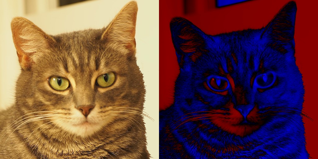

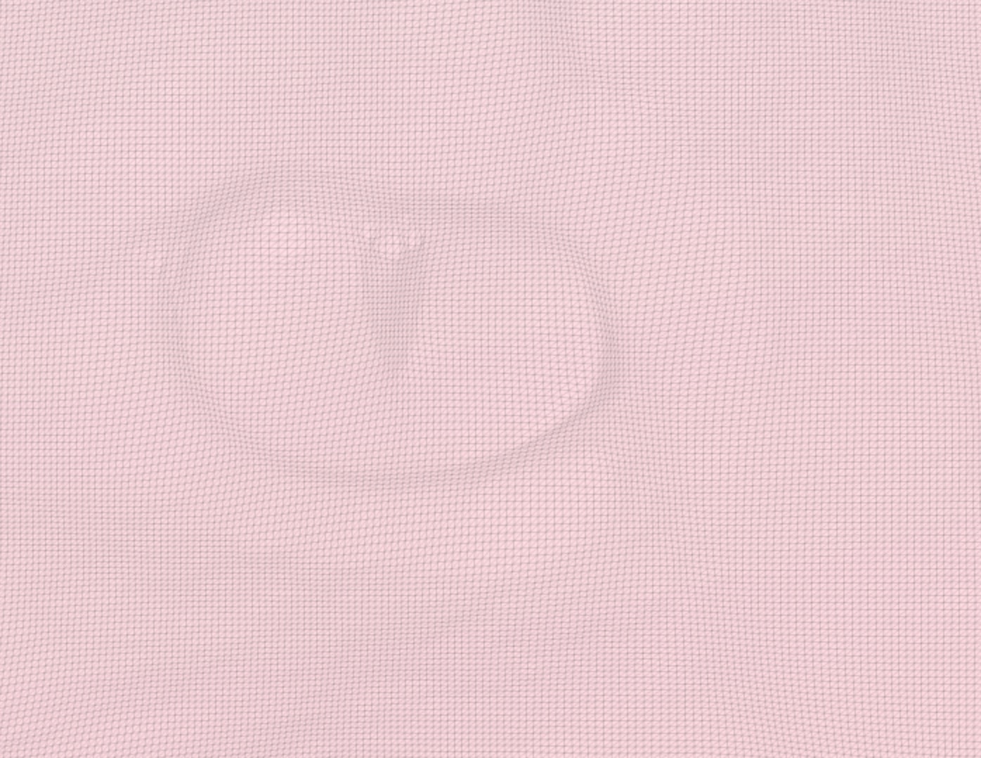
Where I've colorized the loss function so that red areas indicate regions where our grid cells need to grow and blue regions indicate where our grid cells need to shrink.

This image is the loss function L and I'll refer to it a lot.

Stepping to Reduce Loss

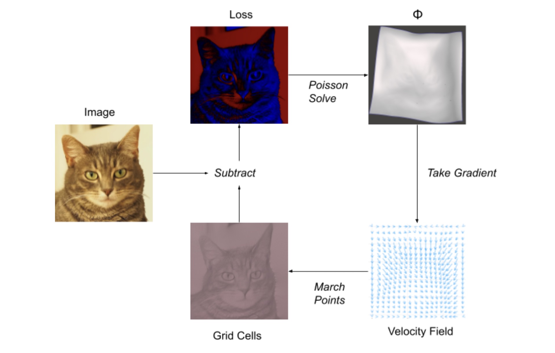
The loss image can be thought of as a scalar field L(x, y). The gradient of a scalar field yields a vector field, which we could call \nabla L(x,y). We can step each grid point slowly in the direction of the gradient field, and in doing so the cells that are too small will get bigger and the cells that are too big will get smaller. Our loss will shrink, and we'll create our image!

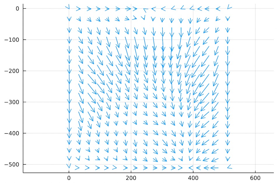
The first thing to do is compute \nabla L and look at the vector field:

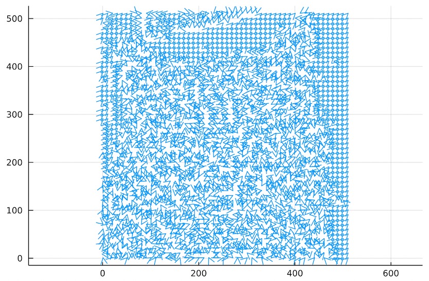
Crap.

\nabla L is a very poorly behaved vector field. It is noisy, discontinuous, and in many places equal to zero.

Almost everywhere, neighboring points need to step in drastically different directions. This creates a situation where improving one cell's loss will necessarily worsen its neighbor's losses, which means that in practice this method can never converge. It's a dead end.

Instead let's draw an analogy to Computational Fluid Dynamics. We need to dilate certain cells and shrink others according to a brightness function. This is similar to modeling compressible air flow where each cell has pressure defined as a pressure function.

If every cell in a 2D grid has some initial pressure, how does the system relax over time? The regions with high pressure expand and the regions of low pressure contract, with regions of middling pressure getting shoved around in a sort of global tug-of-war. Clearly, our problem is analogous.

So, how is this problem solved in CFD simulations? A standard approach is to define a Velocity Potential called \Phi (read: phi). The Velocity Potential \Phi is a scalar field defined at each cell. Its units are meters^2 / second which at first glance is not very easy to interpret. But the reason \Phi is convenient is that its spatial derivatives are measured in meters/second. In other words, the gradient of \Phi gives a vector whose units are velocity:

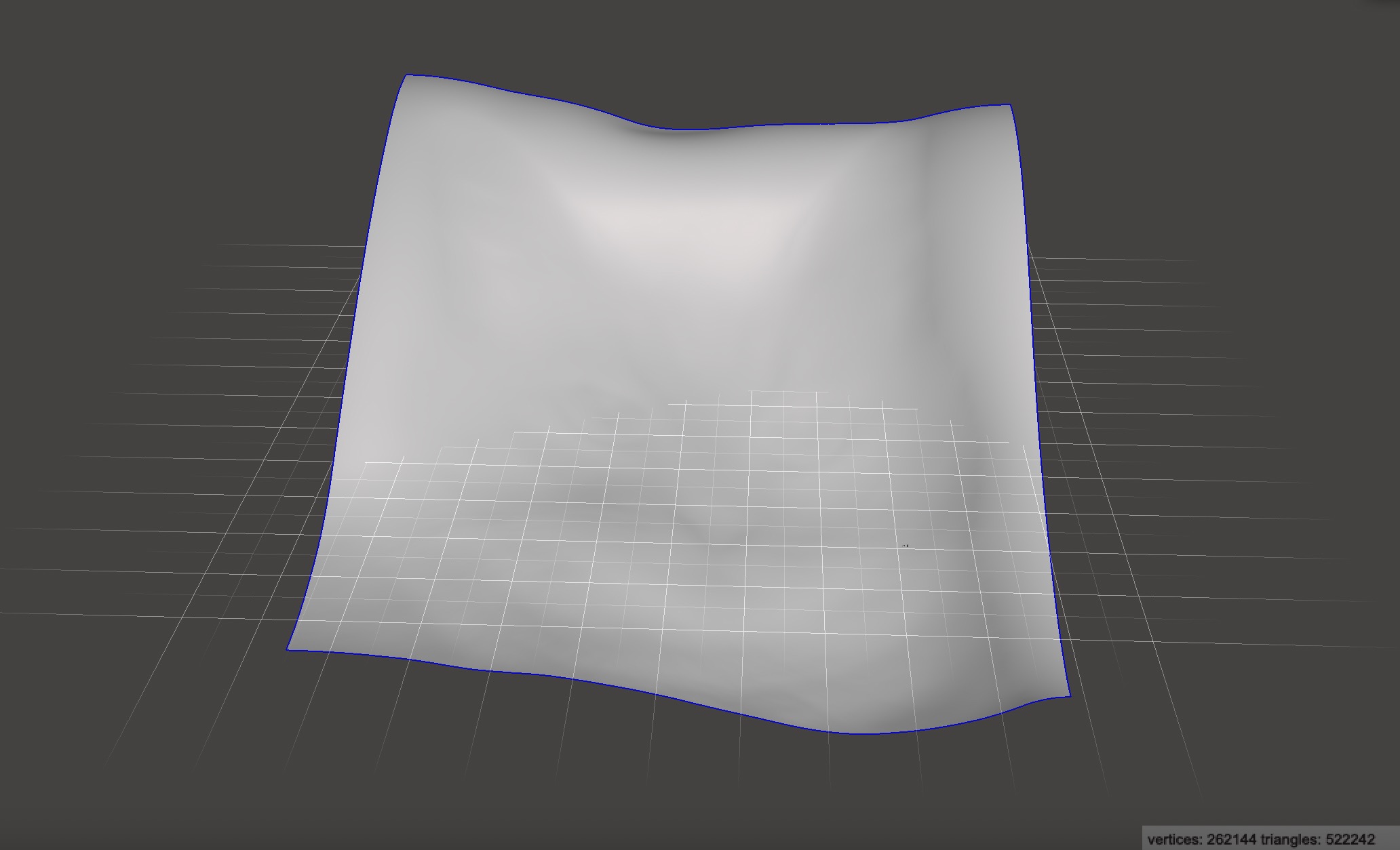
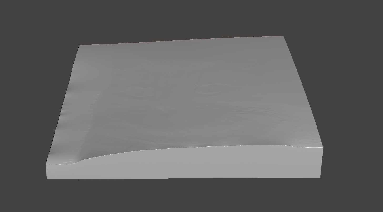
Here is an example \Phi. It is just some scalar field best viewed as a heightmap.

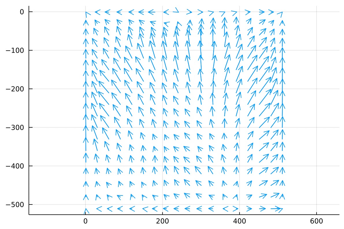
And here is the gradient of that same \Phi. These vectors are velocity vectors that point uphill. If we were performing Computational Fluid Dynamics, these vectors would indicate how fluid might flow from regions of high pressure to regions of low pressure.

Notice how well behaved this vector field is! There is gentle variation across the field but any two neighbors are very similar to each other. None of the arrows pierce the boundary.

In our case we don't have fluid pressure, we have light pressure. Regions in our image which are too bright have high light pressure, which is quantified in our loss function L.

If we can somehow use L to find a \Phi that describes our light pressure distribution, all we need to do is calculate \vec{v} = \nabla \Phi and we'll be able to morph all of our lens grid points according to \vec{v} to decrease our loss!

So how do we find a suitable \Phi? Well, the property we know about each cell is its loss, which encodes how much that cell needs to grow or shrink.

This property, how much a cell grows or shrinks over time as it moves with a velocity field, is called the divergence of that field.

Divergence is written as \nabla \cdot, so in our case, we know that we need to find a velocity field \vec{v} whose divergence equals the loss:

Unfortunately there is no "inverse divergence" operator so we cannot easily invert this equation to find \vec{v} directly. But we can plug equation (1.2) in to equation (1.3) to yield:

Which we read as The divergence of the gradient of the potential field \Phi equals the loss.

This equation comes up surprisingly frequently in many branches of physics and math. It is usually written in a more convenient shorthand:

Which you may recognize as Poisson's Equation!

This is fantastic news because Poisson's equation is extremely easy to solve! If you aren't familiar with it, just think of this step like inverting a big matrix, or numerically integrating an ODE, or finding the square root of a real number. It's an intricate, tedious task that would be painful to do with a paper and pencil, but it's the kind of thing computers are really good at.

Now that we've written down the problem as Poisson's Equation, it is as good as solved. We can use any off the shelf solver, plug in our known L(x, y) using Neumann boundary conditions and boom, and out pops \Phi(x,y) as if by magic.

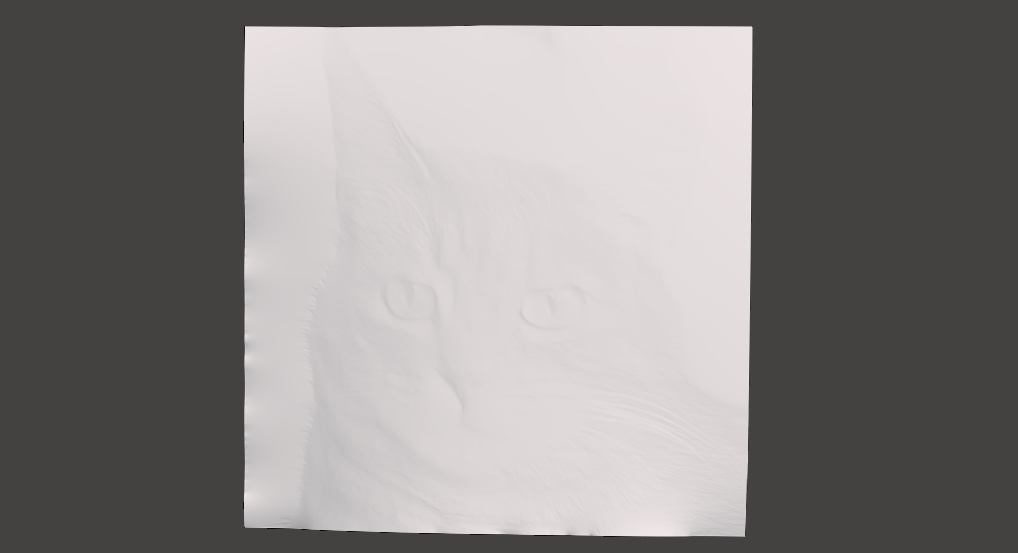
Can you figure out why the cat appears so clearly in this 3D rendering of \Phi? What controls the brightness of each pixel in a render like this?

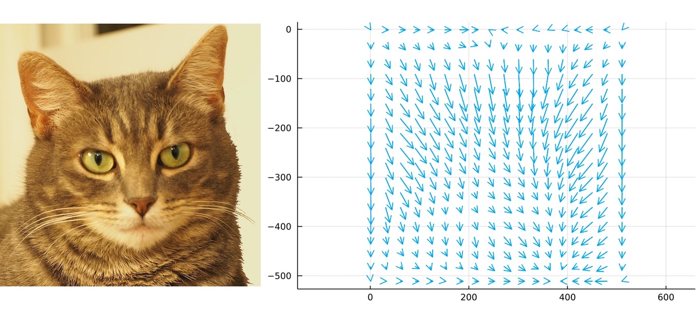
We plug \Phi in to Equation (1.2) to find \vec{v} and we take a look at the vector field:

Disappointingly, it does not look like a kitty to me.

And technically we need to march our points in the direction of negative \nabla L if we want to decrease L. Here's -\nabla L:

But the good news is that this vector field is smooth and well-behaved. We simply march the grid points along this vector field and we'll get exactly what we need.

If you squint you can almost see how the bright background will expand and the cat's dark fur will shrink.

We step all the lens grid points forward some small amount in the direction of -\vec{v}. After morphing the grid a tiny amount we recompute the loss function L, find a new \Phi and new -\vec{v}, and take another small step.

# In Julia-flavored psuedocode
image = read_image("cat.png")
gray = convert_to_grayscale(image)
grid = create_initial_grid(gray.size + 1)

L = compute_loss(gray, grid)

while max(L) > 0.01
    ϕ = poisson_solver(L, "neumann", 0)
    v = compute_gradient(ϕ)
    grid = step_grid(grid, -v)
    L = compute_loss(gray, grid)
end

After three or four iterations the loss gets very small and we've got our morphed cells!

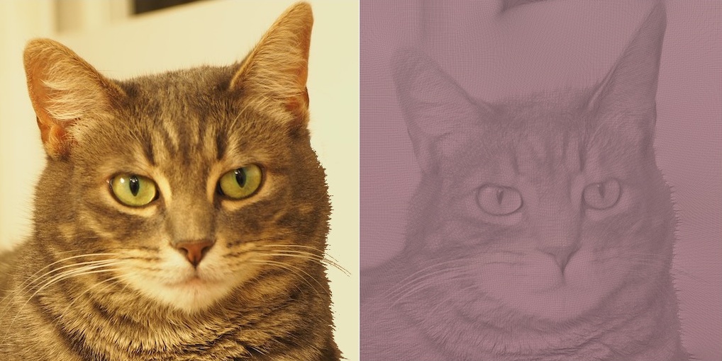
Look at how this cat's chin ballooned out but her nose and forehead shrunk. Her left ear is noticably longer and thinner because the bright background had to grow to take up more light. Her pupils went from oblong to sharp.

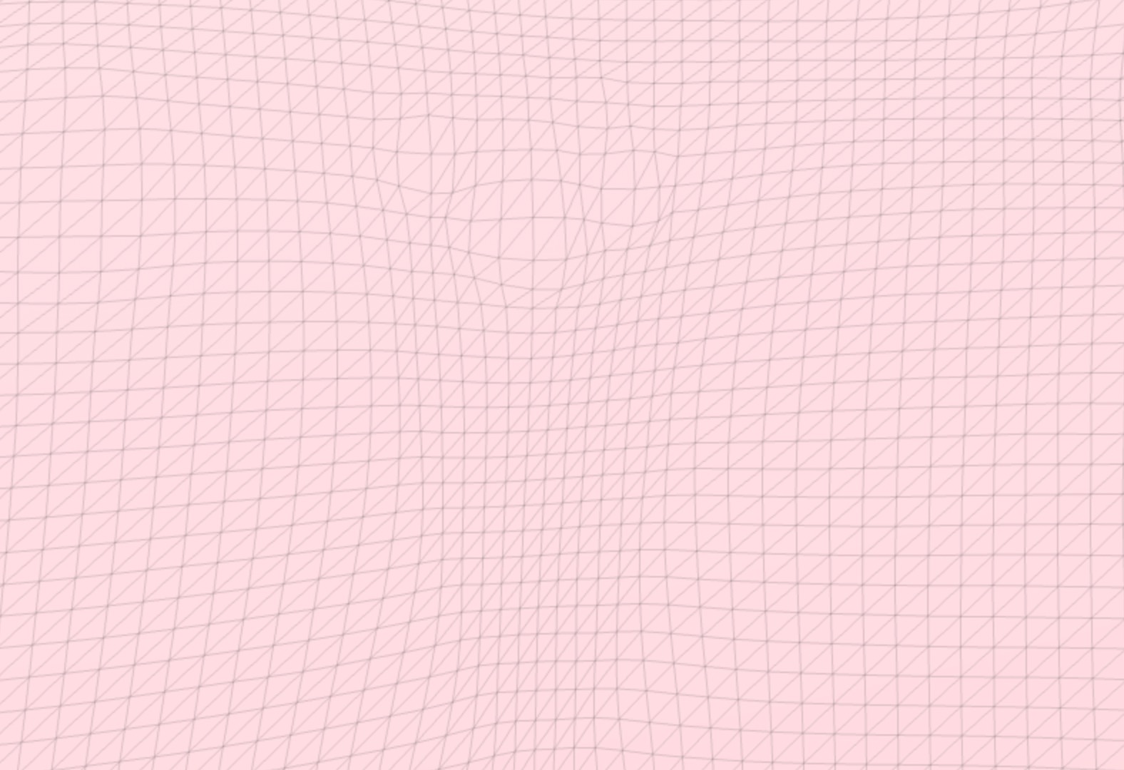
Note that image on the right is just a screenshot of Fusion360's default mesh rendering with the wireframe turned on:

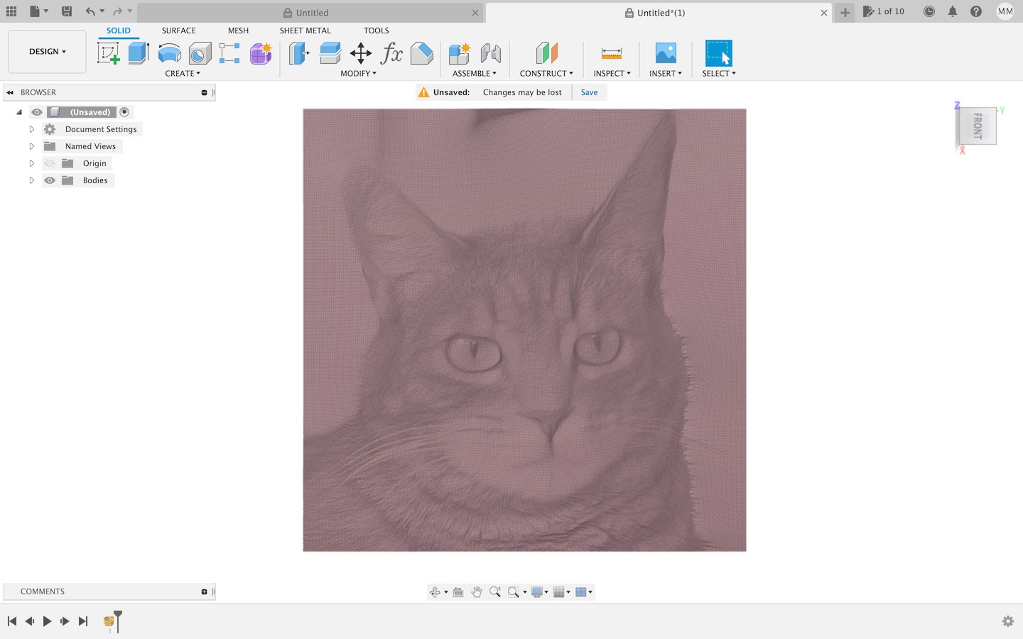
The reason it is darker in some areas is because the mesh is more tightly packed in those areas. Let's zoom in on the eye:

Look at how detailed that is! We've managed to capture even the bright reflections in her eyes. Zooming in further to just the pupil:

We can see the fine structure of the grid cells. Our formulation of the problem is only concerned with cells as quadralaterals. The triangles you see are just an artifact of converting our quadralateral grid into a triangle mesh more suitable for other software to deal with.

So again, in summary:

If we follow these steps we will successfully morph our grid points. Now we've got to do some geometry!

Snell's Law and Normal Vectors

Snell's law tells us how light bends when passing from one material to another.

Where n_1 = 1.49 is the Refractive Index of acrylic and n_2 = 1 is the refractive index of air. If we know \theta_2, Snell's Law gives us \theta_1.

Snell's law is not some arbitrary axiom of physics. It is a direct consequence of Fermat's Principle of Least Time, which is a fascinating and critical link between ray optics and wave optics. But that's a topic for another day.

In our case, each lens cell (i, j) has migrated to position (x, y), and it needs to send its light to the image plane at (u, v), which sits some distance away d.

We start by defining a 3D normal vector \vec{N}(x, y) which everywhere points normal to our heightmap h(x, y).

Normal vectors always point perpendicular to the surface they start on. They generally encode meaning in their direction, not their length, so we're free to scale them to any length that is convenient for our purposes. Very often people choose to make their Normal vectors of length 1.

But if we normalize \vec{N} so that its z coordinate is -1, we can write it:

If you consider just the x and y components, we recognize that

Which is a property often used in computer graphics applications, as well as geospatial applications involving Digital Elevation Models.

Using Snell's Law, a small angle approximation, and a lot of tedious geometry, we find the x and y components of the normal vector \vec{N}:

There is nothing interesting about this derivation so I've skipped it here.

Finding the Heightmap

At this point we have our morphed grid cells and we've found all our surface normals. All we have to do is find a heightmap h(x,y) that has the required surface normals.

Unfortunately, this is not a problem that is solvable in the general case.

We could try to integrate the normals manually, starting at one corner and working our way down the grid, but this method does not usually result in a physically realizable object.

If the integral of the normals running left to right pulls your surface up, but the integral of the normals running top to bottom pulls your surface down, there is just no solution that results in a solid, unbroken surface.

A much better approach is to reach back to equation (2.2), repeated here:

And to take the divergence of both sides:

Do you recognize the form of this equation? Adopting shorthand and swapping sides:

We arrive at yet another instance of Poisson's Equation! We found \vec{N}_{xy} in the previous section, and calculating the divergence of a known vector field is easy:

In code it looks like:

δx = (Nx[i+1, j] - Nx[i, j])
δy = (Ny[i, j+1] - Ny[i, j])
divergence[i, j] = δx + δy

All that's left is to plug our known \nabla \cdot \vec{N}_{xy} in to a Poisson solver with Neumann boundary conditions and out pops h(x, y), ready to use!

Well, there's one thing left to improve. By modifying the height of each point we've actually changed the distance from each lens point to the image, so the lens-image distance is no longer a constant d it is actually a function D(x,y). With our heightmap in hand we can easily calculate:

And repeat the process by calculating new normals using D(x,y) instead of d, which lets us create a new heightmap.

We can loop this process and measure changes to ensure convergence, but in practice just 2 or 3 iterations is all you need:

# In Julia-flavored psuedocode
d = .2 # meters
D = d .* array_of_ones(n, n)

for i in 1:3
    Nx, Ny = compute_normals(grid, D)
    divergence = compute_divergence(Nx, Ny)
    h = poisson_solver(divergence, "neumann", 0)
    D = copy(h)
end

The resulting heightmap can be converted to a solid object by adopting a triangular grid and closing off the back surface.

Note that the image looks mirrored when looking at it head on. That's because the heightmap forms the back surface of the Magic Window. The front surface is factory flat.

The height differences are subtle but certainly enough to get the job done.

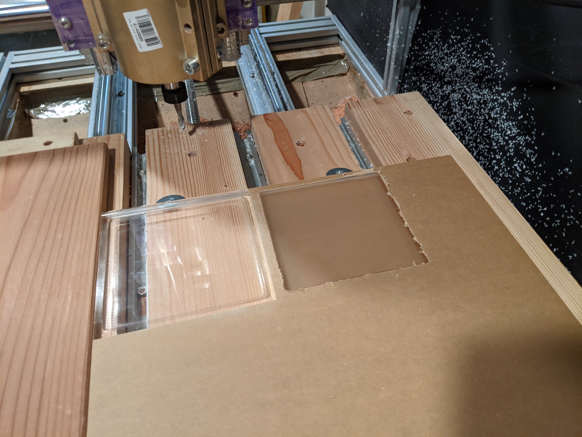
Manufacturing

The process of manufacturing our Magic Window is identical to carving any other 2.5D object.

We bring our object into Fusion360 or any other CAM software. We set up a roughing toolpath left to right, and a finishing toolpath top to bottom just like you find in most tutorials.

Any old CNC router or mill will work. I designed and built my own router last year. If you want to do the same I recommend you start here.

I used a \frac{1}{4} inch diameter, ball-nosed, carbide bit for both roughing and finishing passes, which took 10 minutes and 90 minutes respectively.

After carving the surface finish is rough and transluscent. We need to wet sand using 200, 400, 600, 1000 and 1500 grit sandpapers, then finish with a soft rag and some automotive polish. Sanding and polishing takes about half an hour for a 10 cm \times 10 cm Magic Window.

Acknowledgements

All of the math for this post came from Poisson-Based Continuous Surface Generation for Goal-Based Caustics, a phenomenal 2014 paper by Yue et al. If you continue this work in some way, please cite them.

My Code

My source code is available here. I am a novice at programming in Julia so if you have suggestions for how to improve this code, please reach out or make a pull request!

Caveats: There are a lot of issues with my code. I confuse x and y in several places. I have extra negative signs that I inserted that make the code work but I don't know why. My units and notation are inconsistent throughout. The original paper suggests a better way of calculating loss but I didn't implement it because the naive way was easier, yet I rolled my own mesh utilities and Poisson solver because I enjoyed the challenge.

In short: To me this code is a fun side project. If you want to build a business off of this code you should probably hire someone who knows how to program professionally in Julia.

Licensing

I've posted all my code under the MIT license. Please feel free to use this code for anything you want, including hobbyist, educational, and commercial uses. I only ask that if you make something, please show me!

Except where otherwise attributed, all images in this blog post and the blog post itself are my own work that I license as CC-BY.

The cat in this post is named Mitski and she approves of you using her image as the new standard reference image for image processing papers. It's time to let Lenna retire.

Contact me

If you use my code to make your own Magic Windows, I'd love to see them! I'm on Twitter at @mferraro89. Email me at mattferraro.dev@gmail.com and I will gladly help if you get stuck!

One Last Thing

I know what you're thinking. What about the hologram?!

Does the math above imply that a hologram will always be created, or is this one cat hologram just an incredible coincidence?

Well you see, I've discovered a truly marvelous proof of this, which this website's margin is unfortunately too narrow to contain :)